Using a Deformable Boundaries approach, boundaries of objects or regions in images can be detected and returned as a collection of curves. These algorithms start from initial guesses of curves, and deform them iteratively towards the correct boundaries, guided by energy minimization principles. Scikit-shape
Scikit-shape includes two approaches for this: shape optimization of curve objects (explicit Lagrangian approach), evolution of a phase field function embedding the curves (implicit Eulerian approach).
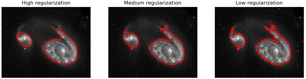
skshape.segmentation.segment_phase_field function is used to produce regions with smooth regular boundaries. The regularity of the boundaries can be adjusted by setting lower or higher ``data_weight``. This example shows different degrees of regularization on the boundaries of the galaxies segmented. In the first example, the ``data_weight`` is low, so regularization is stronger, and this results in smooth boundaries. In the second example, the ``data_weight`` is higher, so the boundaries are less smooth. In the third example, the ``data_weight`` is highest, so the boundaries are very irregular, but they fit the data more tightly, i.e. overfitting as a natural result of the high ``data_weight``.”
Download the Python code for Deformable Boundaries.


import matplotlib.pyplot as plt
from skimage.measure import find_contours
from skshape.image.segmentation import segment_phase_field
def plot_boundaries(image, curves, plot_no, title_text):
plt.subplot(1,3,plot_no); plt.imshow(image)
for c in curves:
plt.plot( c[:,1], c[:,0], 'r-', linewidth=2 )
plt.title('Deformable Boundaries'); plt.axis('off')
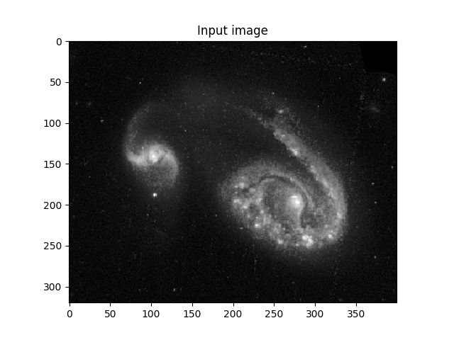
I = plt.imread('two_galaxies.png')
plt.figure(); plt.imshow(I); plt.gray();
plt.title('Input image'); plt.show()
plt.figure()
init_segmentation = (I > 0.2)
high_reg_result = segment_phase_field(I, init_segmentation, data_weight=100)
boundaries = find_contours(high_reg_result, 0.5)
plot_boundaries(I, boundaries, 1, 'High Regularization')
med_reg_result = segment_phase_field(I, init_segmentation, data_weight=500)
boundaries = find_contours(med_reg_result, 0.5)
plot_boundaries(I, boundaries, 2, 'Medium Regularization')
low_reg_result = segment_phase_field(I, init_segmentation, data_weight=2000)
boundaries = find_contours(low_reg_result, 0.5)
plot_boundaries(I, boundaries, 3, 'Low Regularization')
plt.show()