skshape.numerics.fem package

Submodules

skshape.numerics.fem.curve_fem module

class skshape.numerics.fem.curve_fem.ReferenceElement[source]

Bases: object

eval_basis_fct(quad)[source]

eval_basis_fct_products(quad)[source]

interpolate(u, s, mask=None, coarsened=False)[source]

Interpolates a given data vector at s on elements of the curve.

Interpolates a given vector u of data points linearly at the local coordinate s on selected elements of the curve.

The data vector u can be scalar-valued, i.e. an array of size n (= curve.size()) with a single value for each node of the curve, or vector-valued with size d x n, or matrix-valued with size d1 x d2 x n.

For example, if u is the NumPy array [1.0, 2.0, 3.0, 4.0] and s = 0.25, and if the interpolation is performed for all elements (mask = None, coarsened = False), then the interpolation is computed by

[ (1.0 - 0.25) * 1.0 + 0.25 * 2.0,
(1.0 - 0.25) * 2.0 + 0.25 * 3.0, (1.0 - 0.25) * 3.0 + 0.25 * 4.0, (1.0 - 0.25) * 4.0 + 0.25 * 1.0 ]

and the return value is the NumPy array: u_at_s = [ 1.25, 2.25, 3.25, 3.25 ]

If in addition the mask array is specified as [0,2], then the interpolation is computed for 0th and 2nd elements only,

u_at_s = [ 1.25, 3.25 ]

If mask = [1] and coarsened = True, then the interpolation is for the 1st element when is coarsened (combined with the 2nd element; therefore the data comes from the 1st and the 3rd nodes and u_at_s = [ (1.0 - 0.25) * 2.0 + 0.25 * 4.0 ] = [ 2.5 ].

If mask = None and coarsened = True, then all elements are coarsened and only the elements with nodes (0,2) and (2,0) remain with their data

u_at_s = [ (1.0 - 0.25) * 1.0 + 0.25 * 3.0,

(1.0 - 0.25) * 3.0 + 0.25 * 1.0 ]

= [ 1.5, 2.5 ]

In the case of odd number of elements, the last element is not coarsened.

Parameters

u (NumPy array) – The data vector, a float array of size n or d x n or d1 x d2 x n, where n is the number of nodes on the curve.
s (float) – The local coordinate on the element, a scalar number between 0 and 1 (included).
mask (NumPy array, optional) – One-dimensional array of integers storing the indices of the elements where the global coordinates for s will be computed, the integers should be in the range: 0, …, curve.size()-1.
coarsened (bool, optional) – An argument denoting whether we compute the global coordinates for the current elements of the given curve (coarsened = False) or for the elements that result from coarsening the current elements (coarsened = True).

Returns

u_at_s – elements, a NumPy float array with same size as u.

Return type

The value of interpolation at s on all selected

Raises

ValueError – Error if u.ndim > 3.

local_to_global(s, curve, mask=None, coarsened=False)[source]

Returns the global coordinate for all elements at local coordinate s.

Given a curve (which stores the information for all its elements) and a local coordinate s from [0,1] on the reference element, this function returns the corresponding global coordinates X on all the elements. If mask, an array of indices of some of the elements, is given, then the global coordinates on only the elements specified by the indices in mask is given. If coarsened is set to True, then the global coordinates are not computed for the current elements. They are computed for the elements that would result from coarsening the current elements.

For example, if the curve is the square with the corner nodes {(-1,-1), (1,-1), (1,1), (-1,1)} ordered counterclockwise and s = 0.25, then the corresponding global coordinate vector is X = {(-0.5,-1.0), (1.0,-0.5), (0.5,1.0), (-1.0,0.5)}, more specifically the NumPy array:

X = [[-0.5, 1.0, 0.5, -1.0], [-1.0, -0.5, 1.0, 0.5]].

If in addition the mask array is specified as [0,2], then the global coordinates are X = {(-0.5,-1.0), (0.5,1.0)}, the coordinates of only the 0th and 2nd elements.

If mask = [1] and coarsened = True, then the global coordinates are sought for the coarse element resulting from the coarsening of the element 1 (and 2). When element 1 is coarsened, the corresponding coarse element is (1,-1)-(-1,1) and the global coordinate on this element for s = 0.25 is X = (0.5,-0.5). So the return vector is the NumPy array: X = [[0.5],[-0.5]].

If mask = None and coarsened = True, then all the elements are coarsened and the global coordinates are returned for these coarsened elements. In the square example, the first element with nodes (0,1) will be combined with the second element (1,2) to get (0,2). Similarly, the third and fourth are combined into (2,0). Thus the new coarse elements have the coordinates (-1,-1)-(1,1) and (1,1)-(-1,-1) respectively. Then global coordinates for s = 0.25 are (-0.5,-0.5) and (0.5,0.5). So the return vector is the NumPy array:

X = [[-0.5,0.5],[-0.5,0.5]]

In the case of odd number of elements, the last element is not coarsened.

Parameters

s (float) – The local coordinate on the element, a scalar number between 0 and 1 (included).
curve (Curve object) –
mask (NumPy array, optional) – An optional one-dimensional array of integers storing the indices of the elements where the global coordinates for s will be computed, the integers should be in the range 0, …, curve.size()-1.
coarsened (bool, optional) – An optional argument denoting whether we compute the global coordinates for the current elements of the given curve (coarsened = False) or for the elements that result from coarsening the current elements (coarsened = True).

Returns

X – A two-dimensional array of the global coordinates on all elements corresponding to the given local coordinate s, size of X will be 2 x curve.size().

Return type

NumPy array

quadrature(degree=None, order=None)[source]

random_elements(grid_size, diameter)[source]

skshape.numerics.fem.curve_fem.load_vector(curves, f=None, f2=None, quad=None)[source]

skshape.numerics.fem.curve_fem.mass_matrix(curves)[source]

skshape.numerics.fem.curve_fem.normal_matrix(curves, normal_component)[source]

skshape.numerics.fem.curve_fem.pwconst_weighted_mass_matrix(curves, weight)[source]

skshape.numerics.fem.curve_fem.rand(d0, d1, ..., dn)

Random values in a given shape.

Note

This is a convenience function for users porting code from Matlab, and wraps random_sample. That function takes a tuple to specify the size of the output, which is consistent with other NumPy functions like numpy.zeros and numpy.ones.

Create an array of the given shape and populate it with random samples from a uniform distribution over [0, 1).

Parameters

d0 (int, optional) – The dimensions of the returned array, must be non-negative. If no argument is given a single Python float is returned.
d1 (int, optional) – The dimensions of the returned array, must be non-negative. If no argument is given a single Python float is returned.
.. (int, optional) – The dimensions of the returned array, must be non-negative. If no argument is given a single Python float is returned.
dn (int, optional) – The dimensions of the returned array, must be non-negative. If no argument is given a single Python float is returned.

Returns

out – Random values.

Return type

ndarray, shape (d0, d1, ..., dn)

skshape.numerics.fem.domain2d_fem module

class skshape.numerics.fem.domain2d_fem.ReferenceElement[source]

Bases: object

local_to_global(s, mesh, mask=None, coarsened=False)[source]

quadrature(degree=None, order=None)[source]

random_elements(grid_size, diameter)[source]

Returns a Domain2d mesh made up of random elements about pixel size.

Given a grid specified by grid_size and diameter, this function creates and returns a Domain2d mesh composed of random elements scattered around the physical domain defined by the grid. All the random elements are roughly half the size of a single pixel of the grid, about 0.5 * (diameter / min(grid_size))**2.

Parameters

grid_size (tuple of two integers) – A pair of two integers that gives the size or resolution of the grid. By grid, we mean a set of evenly-spaced points, such as the pixels in an image grid.
diameter (float) – The length of the ‘shortest’ side of the grid, the shortest edge of the rectangle

Returns

mesh – An instance of a Domain2d class made up of min(grid_size) random elements, each of which is about the size of a pixel of the grid specified by grid_size or diameter.

Return type

Domain2d object

skshape.numerics.fem.domain2d_fem.lognormal(mean=0.0, sigma=1.0, size=None)

Draw samples from a log-normal distribution.

Draw samples from a log-normal distribution with specified mean, standard deviation, and array shape. Note that the mean and standard deviation are not the values for the distribution itself, but of the underlying normal distribution it is derived from.

Note

New code should use the lognormal method of a default_rng() instance instead; see random-quick-start.

Parameters

mean (float or array_like of floats, optional) – Mean value of the underlying normal distribution. Default is 0.
sigma (float or array_like of floats, optional) – Standard deviation of the underlying normal distribution. Must be non-negative. Default is 1.
size (int or tuple of ints, optional) – Output shape. If the given shape is, e.g., (m, n, k), then m * n * k samples are drawn. If size is None (default), a single value is returned if mean and sigma are both scalars. Otherwise, np.broadcast(mean, sigma).size samples are drawn.

Returns

out – Drawn samples from the parameterized log-normal distribution.

Return type

ndarray or scalar

See also

scipy.stats.lognorm(): probability density function, distribution, cumulative density function, etc.
Generator.lognormal(): which should be used for new code.

Notes

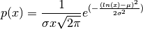
A variable x has a log-normal distribution if log(x) is normally distributed. The probability density function for the log-normal distribution is:

$p(x) = \frac{1}{\sigma x \sqrt{2\pi}} e^{(-\frac{(ln(x)-\mu)^2}{2\sigma^2})}$

where $\mu$ is the mean and $\sigma$ is the standard deviation of the normally distributed logarithm of the variable. A log-normal distribution results if a random variable is the product of a large number of independent, identically-distributed variables in the same way that a normal distribution results if the variable is the sum of a large number of independent, identically-distributed variables.

References

1: Limpert, E., Stahel, W. A., and Abbt, M., “Log-normal Distributions across the Sciences: Keys and Clues,” BioScience, Vol. 51, No. 5, May, 2001. https://stat.ethz.ch/~stahel/lognormal/bioscience.pdf
2: Reiss, R.D. and Thomas, M., “Statistical Analysis of Extreme Values,” Basel: Birkhauser Verlag, 2001, pp. 31-32.

Examples

Draw samples from the distribution:

>>> mu, sigma = 3., 1. # mean and standard deviation
>>> s = np.random.lognormal(mu, sigma, 1000)

Display the histogram of the samples, along with the probability density function:

>>> import matplotlib.pyplot as plt
>>> count, bins, ignored = plt.hist(s, 100, density=True, align='mid')

>>> x = np.linspace(min(bins), max(bins), 10000)
>>> pdf = (np.exp(-(np.log(x) - mu)**2 / (2 * sigma**2))
...        / (x * sigma * np.sqrt(2 * np.pi)))

>>> plt.plot(x, pdf, linewidth=2, color='r')
>>> plt.axis('tight')
>>> plt.show()

Demonstrate that taking the products of random samples from a uniform distribution can be fit well by a log-normal probability density function.

>>> # Generate a thousand samples: each is the product of 100 random
>>> # values, drawn from a normal distribution.
>>> b = []
>>> for i in range(1000):
...    a = 10. + np.random.standard_normal(100)
...    b.append(np.product(a))

>>> b = np.array(b) / np.min(b) # scale values to be positive
>>> count, bins, ignored = plt.hist(b, 100, density=True, align='mid')
>>> sigma = np.std(np.log(b))
>>> mu = np.mean(np.log(b))

>>> x = np.linspace(min(bins), max(bins), 10000)
>>> pdf = (np.exp(-(np.log(x) - mu)**2 / (2 * sigma**2))
...        / (x * sigma * np.sqrt(2 * np.pi)))

>>> plt.plot(x, pdf, color='r', linewidth=2)
>>> plt.show()

skshape.numerics.fem.domain2d_fem.rand(d0, d1, ..., dn)

Random values in a given shape.

Note

This is a convenience function for users porting code from Matlab, and wraps random_sample. That function takes a tuple to specify the size of the output, which is consistent with other NumPy functions like numpy.zeros and numpy.ones.

Create an array of the given shape and populate it with random samples from a uniform distribution over [0, 1).

Parameters

d0 (int, optional) – The dimensions of the returned array, must be non-negative. If no argument is given a single Python float is returned.
d1 (int, optional) – The dimensions of the returned array, must be non-negative. If no argument is given a single Python float is returned.
.. (int, optional) – The dimensions of the returned array, must be non-negative. If no argument is given a single Python float is returned.
dn (int, optional) – The dimensions of the returned array, must be non-negative. If no argument is given a single Python float is returned.

Returns

out – Random values.

Return type

ndarray, shape (d0, d1, ..., dn)

skshape.numerics.fem.grid_fem module

class skshape.numerics.fem.grid_fem.ReferenceElement[source]

Bases: object

interpolate(u, s)[source]

local_to_global(s, mesh, mask=None, coarsened=False)[source]

quadrature(degree=None, order=None)[source]

skshape.numerics.fem.grid_fem.assemble_system_matrix(grid, alpha, beta)[source]

skshape.numerics.fem.grid_fem.ellipt_matvec(grid, alpha, beta, u)[source]

skshape.numerics.fem.grid_fem.inv_diag_ellipt_matvec(grid, alpha, beta, u)[source]

skshape.numerics.fem.grid_fem.load_vector(grid, f)[source]

skshape.numerics.fem.grid_fem.solve_elliptic_pde(grid, alpha, beta, f, g=0.0)[source]

skshape.numerics.fem package

Submodules

skshape.numerics.fem.curve_fem module

skshape.numerics.fem.domain2d_fem module

skshape.numerics.fem.grid_fem module

Module contents

Table of Contents